使用numpy实现逻辑回归对IRIS数据集二分类
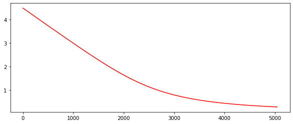
使用numpy实现逻辑回归对IRIS数据集二分类,使用对数似然损失(Log-likelihood Loss),并显示训练后loss变化曲线。
知识储备如下:
- 逻辑回归Logistic Regression
- 对数似然损失
- IRIS数据集介绍
- np.concatenate使用
知识储备
逻辑回归Logistic Regression
名字虽然叫回归,但是一般处理的是分类问题,尤其是二分类,比如垃圾邮件的识别,推荐系统,医疗判断等,因为其逻辑与实现简单,在工业界有着广泛的应用。
优点:
- 实现简单,计算代价不高,易于理解和实现, 广泛的应用于工业问题上;
- 分类时计算量非常小,速度很快,存储资源低;
缺点:
- 容易欠拟合,当特征空间很大时,逻辑回归的性能不是很好;
- 不能很好地处理大量多类特征或变量;
对数似然损失
对数损失, 即对数似然损失(Log-likelihood Loss), 也称逻辑斯特回归损失(Logistic Loss)或交叉熵损失(cross-entropy Loss), 是在概率估计上定义的。它常用于(multi-nominal, 多项)逻辑斯特回归和神经网络,以及一些期望极大算法的变体,可用于评估分类器的概率输出。可参考对数损失函数(Logarithmic Loss Function)的原理和 Python 实现了解详情

损失函数:
梯度计算:
权重更新:
IRIS数据集介绍
该数据集包含4个特征变量,1个类别变量。iris每个样本都包含了4个特征:花萼长度,花萼宽度,花瓣长度,花瓣宽度,以及1个类别变量(label)。详情见加载数据
np.concatenate使用
1 | a = np.array([[1, 2],[3, 4]]) |
array([[1, 2],
       [3, 4],
       [5, 6]])
1 | np.concatenate((a, b.T), axis = 1) |
array([[1, 2, 5],
       [3, 4, 6]])
加载数据
1 | import matplotlib.pyplot as plt |
1 | dataset = load_iris() |
inputs.shape: (150, 4)
target.shape: (150,)
labels: {0, 1, 2}
1 | target |
array([0, 0, 0, 0, 0, 0, 0, 0, 0, 0, 0, 0, 0, 0, 0, 0, 0, 0, 0, 0, 0, 0,
       0, 0, 0, 0, 0, 0, 0, 0, 0, 0, 0, 0, 0, 0, 0, 0, 0, 0, 0, 0, 0, 0,
       0, 0, 0, 0, 0, 0, 1, 1, 1, 1, 1, 1, 1, 1, 1, 1, 1, 1, 1, 1, 1, 1,
       1, 1, 1, 1, 1, 1, 1, 1, 1, 1, 1, 1, 1, 1, 1, 1, 1, 1, 1, 1, 1, 1,
       1, 1, 1, 1, 1, 1, 1, 1, 1, 1, 1, 1, 2, 2, 2, 2, 2, 2, 2, 2, 2, 2,
       2, 2, 2, 2, 2, 2, 2, 2, 2, 2, 2, 2, 2, 2, 2, 2, 2, 2, 2, 2, 2, 2,
       2, 2, 2, 2, 2, 2, 2, 2, 2, 2, 2, 2, 2, 2, 2, 2, 2, 2])
1 | values = [np.sum(target == 0), np.sum(target == 1), np.sum(target == 2)] |

关于参数train_test_split的random_state的解释:
Controls the shuffling applied to the data before applying the split. Pass an int for reproducible output across multiple function calls.
random_state即随机数种子,目的是为了保证程序每次运行都分割一样的训练集和测试集。否则,同样的算法模型在不同的训练集和测试集上的效果不一样。
1 | from sklearn.model_selection import train_test_split |
(70, 4) (30, 4) (70, 1) (30, 1)
1 | # add one feature to x |
(70, 5) (30, 5)
定义模型
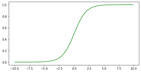
1 | def sigmoid(x): |
[<matplotlib.lines.Line2D at 0x28f77053348>]
1 | compute_loss = lambda pred_y, y: np.mean(-y * np.log(pred_y)-(1-y) * np.log(1-pred_y)) |
[<matplotlib.lines.Line2D at 0x28f77053508>]
测试样例
1 | # 测试 |
the accary of model is 100.0
1 | print(pre_test_y.reshape(1,-1)) |
[[0. 1. 0. 1. 1. 1. 0. 1. 1. 1. 1. 1. 1. 0. 0. 0. 0. 0. 0. 0. 0. 1. 0. 1. 0. 0. 0. 1. 1. 1.]]
[[0 1 0 1 1 1 0 1 1 1 1 1 1 0 0 0 0 0 0 0 0 1 0 1 0 0 0 1 1 1]]